top of page

Contents
Examining Graphs of Functions

Zeros of Functions: Inputs to a given function that result in an output of zero. Zeros of a function are the x-intercepts of the function’s graph.

Increasing: Rises from left to right.
Decreasing: Descends from left to right.
Constant: Stays the same.

Relative Maximum: The highest point in an interval.
Relative Minimum: The lowest point in an interval.
The relative maxima and minima are the turning points of the graph where the function changes from increasing to decreasing or vice versa.
Difference Quotient

Average Rate of Change: Slope.


Difference Quotient: The slope of a secant line that passes through a curve.
Secant Line: A line that intersects two or more points on a curve.
Symmetry
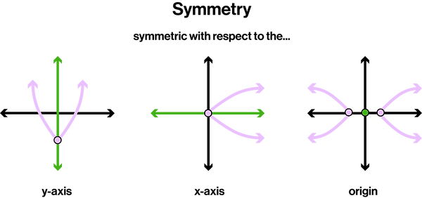
Symmetry: A reflection across a line or point.

Even Functions: Functions that are symmetric with respect to the y-axis.
Odd Functions: Functions that are symmetric with respect to the origin.
Transformations


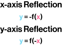


Transformation: A graph is changed by shifting, reflecting, stretching, and/or shrinking.
Greatest Integer Function

Greatest Integer Function: A function of the form f(x)=[x], where f(x) is equal to the greatest integer less than or equal to x.
Polynomial Functions

Polynomial functions are continuous, smooth, and have a domain of all real numbers (-∞ , ∞).

Leading-Term Test: A test used to determine the behavior of a polynomial's graph.

The degree of a polynomial will dictate the number of possible zeros and the number of turning points.

Indeterminate Value Theorem: A theorem that can be used to determine if a real zero exists between two x values.

The factored form of a polynomial can directly express that polynomial’s zeros.

Rational Roots Test: A test that is used to determine the zeros of a polynomial function if the polynomial function has integer coefficients.

Real-number zeros can also be found by graphing the polynomial function.
.png)

Polynomial division can be used to check if one polynomial is a factor of another. If the remainder is zero, the divisor is a factor of the dividend. Polynomial division can be paired with other methods to find a polynomial's zeros.

Other methods learned in elementary and intermediate algebra may be required to find the zeros of a polynomial function.

Zeros can be used to find a corresponding polynomial.

If a complex number is found to be a zero of a polynomial function with real coefficients, its conjugate will also be a zero.

Certain irrational zeros will occur in pairs for polynomial functions with rational coefficients.


Multiplicity: The number of times a factor appears in a polynomial’s factored form.
Tangent: A straight line that touches a curve at a point.
Rational Functions

Rational Functions: Functions that are a quotient of two polynomials.
The domain of a rational function includes all real numbers, except those that make the denominator zero.

Vertical Asymptotes: Exist at any x-values that make the polynomial in the denominator zero.
.png)
.png)
Horizontal Asymptotes: Exist at y = 0 when the degree of the numerator is less than the degree of the denominator. A horizontal asymptote can also exist when the degree of the numerator is equal to the degree of the denominator. When the degrees are equal, the leading coefficients dictate the location of the horizontal asymptote.


Oblique Asymptotes: Exist when the degree of the numerator is one greater than the degree of the denominator.
Multiple asymptotes can exist for a given rational function; however, there can only be one horizontal asymptote or one oblique asymptote. A horizontal asymptote will never occur with an oblique asymptote and vice versa.
Trigonometric Functions

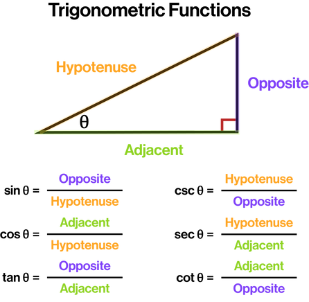

Acute Angle: An angle with a measure greater than 0° and less than 90°. Acute angles are typically denoted by Greek letters.
Hypotenuse: The side opposite the right angle.

The cosecant, secant, and cotangent functions are the reciprocals of the sine, cosine, and tangent functions.


Pythagorean Equation: An equation used to determine the side lengths of a right triangle.

Cofunction Identities: Identities that relate trigonometric functions and their complementary angles.

To solve a triangle, all of its sides and angles must be determined.
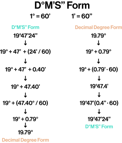
D°M’S’’ Form (Degrees, Minutes, Seconds): A classical way of expressing the measurement of an angle.
Decimal Degree Form: The standard way of expressing the measurement of an angle.
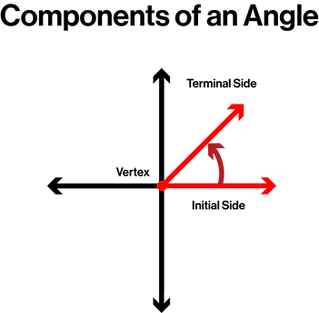
Vertex: The common endpoint of the two rays of an angle.
Initial Side: The ray at the beginning of the rotation.
Terminal Side: The ray at the end of the rotation.
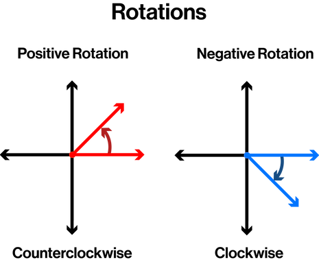
Positive Rotation: A counterclockwise rotation.
Negative Rotation: A clockwise rotation.

Coterminal Angles: Angles that have the same terminal side. Coterminal angles can be found by adding or subtracting multiples of 360° from the angle of interest.


The trigonometric functions can be applied to angles of any size.

.png)
Bearing: Giving direction.

Radians: An alternate unit of measurement for angles.
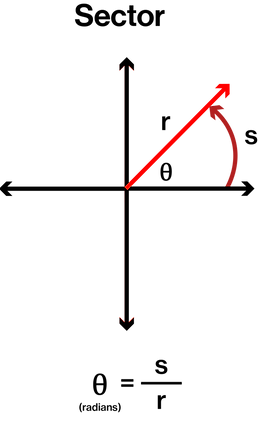
The arc length formula from geometry can be used to find the radius, arc length, or radians of a given angle.

The linear and angular speed formulas can be used for questions related to speed and rotational motion.

Circular Functions: Trigonometric functions with domains consisting of real numbers.

Unit Circle: A tool used to find the most frequently used trigonometric function values and their associated radians or degrees.

The sine and cosine functions have two output values per cycle. For some questions, all outputs for a cycle will be requested.
Graphs of Trigonometric Functions


The domain of the sine and cosine functions is (-∞ , ∞). The range of the sine and cosine functions is [-1, 1]. The sine function is odd, and the cosine function is even.

Periodic Functions: Functions with a repeating pattern. For a function of the form f(s + p), p is the period.

Amplitude: One-half the distance between a periodic function’s maximum and minimum values. Amplitude is always positive.

The domain of the tangent function is all real numbers except π/2 + kπ, where k is any integer. The range of the tangent function is (-∞ , ∞). The tangent function has a period of π and does not have an amplitude.

The domain of the cotangent function is all real numbers except kπ, where k is any integer. The range of the cotangent function is (-∞ , ∞). The cotangent function has a period of π and does not have an amplitude.

The domain of the cosecant function is all real numbers except kπ, where k is any integer. The range of the cosecant function is (-∞ , -1] ∪ [1 , ∞). The cosecant function has a period of 2π and does not have an amplitude.

The domain of the secant function is all real numbers except π/2 + kπ, where k is any integer. The range of the secant function is (-∞ , -1] ∪ [1 , ∞). The secant function has a period of 2π and does not have an amplitude.

The sine and cosine functions can be transformed by changing the A, B, C, and D constants.
Trigonometric Identities


Identity: An equation that is true for all possible replacements of the variables. Identities can be used to manipulate and simplify trigonometric expressions and equations.
Trigonometric Inverses


The inverse trigonometric functions can be used to solve trigonometric equations.
Law of Sines and Law of Cosines
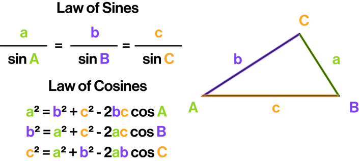
The law of sines and the law of cosines, learned in geometry, can be used to solve oblique triangles.
Complex Numbers (Trigonometric Notation)
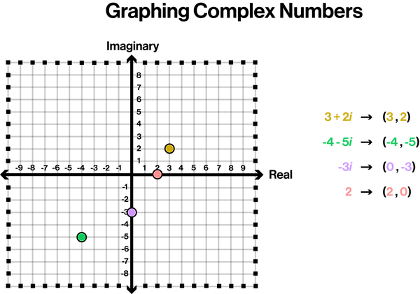
Complex numbers can be graphed on a coordinate plane; however, the x-axis is switched to the real axis, and the y-axis is switched to the imaginary axis.

The absolute value of a complex number is its distance from the origin on a coordinate plane.


Trigonometric Notation: An alternative notation for complex numbers that uses trigonometric functions. A graphing calculator can be used to convert complex numbers in trigonometric notation to standard notation.


Operations can be applied to complex numbers in their trigonometric notation form.
Polar Coordinates


Polar Coordinates: The radius and angle are used as coordinates. Polar coordinates are graphed on a polar graph.

Polar Equation: An equation that involves polar coordinates. A graphing calculator can graph a polar equation when the graph type is changed to r =.
Vectors

Vector: A quantity with magnitude and direction that is represented by a directed line segment.
Equivalent Vectors: Vectors with the same magnitude and direction; however, equivalent vectors don’t need to occupy the same location.


Vectors can be added together using the method learned in geometry. Alternatively, the initial points of the vectors can be placed together, and the diagonal of the parallelogram is equivalent to the sum of the vectors.

If a vector is converted to component form, as learned in geometry, its length can be determined. The length of a vector is the same as its magnitude.

Operations can be applied to component form vectors.

Unit Vector: A vector of length one.


Linear Combination: Multiplying each vector by a scalar and then adding the results together.

Dot Product: A scalar that is the product of two vectors. A dot product can be used to determine the angle between two vectors.
Matrices (Continued)

Gaussian Elimination: A method of solving systems of equations using a corresponding matrix. The goal of Gaussian Elimination is to transform the matrix into row-echelon form.

Gauss–Jordan Elimination: A method of solving systems of equations using a corresponding matrix. The goal of Gauss–Jordan Elimination is to transform the matrix into reduced row-echelon form.

The inverse of a matrix can be found using a graphing calculator.

If a matrix is invertible, it can be used to solve a corresponding system of equations. A graphing calculator is recommended to hasten the process of determining the solution.


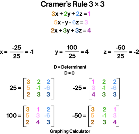
Cramer’s Rule: A method used to solve systems of equations using determinants.
Conic Sections

Conic Section: A curve that is the result of a plane intersecting a cone.

Conic sections can be defined using second-degree equations.


Parabola: The set of all points in a plane that are equidistant from the directrix and the focus.

Circle: The set of all points in a plane that are a fixed distance from the center.

Ellipse: The set of all points in a plane whose sum of their distances from the foci is constant.

Hyperbola: The set of all points in a plane whose absolute value of the difference of their distances from the foci is constant.
Practice Sheets
bottom of page