
Contents
Types of Functions


Functions


Domain: The set of all first coordinates of the ordered pairs in a function.
Range: The set of all second coordinates of the ordered pairs in a function.
Function: A correspondence between the domain and range such that each member of the domain corresponds to only one member of the range.

Set Notation: A notation used to describe the elements of a function.

Functions can be visualized by graphing each of the function’s ordered pairs.

Functions are named using lowercase or uppercase letters.

.png)
Function Notation: A notation used to describe the correspondence between an element of the domain, an input, and its corresponding range element, an output.
The notation f(x) is read as “f of x” or “f at x.”

Vertical Line Test: A vertical line cannot cross the graph of a function more than once. If the line crosses the graph more than once, the graph does not belong to a function.
Relation: A correspondence between the domain and the range such that each member of the domain corresponds to at least one member of the range.

Functions can be described by equations.


An important aspect of characterizing a function is defining its domain and range.

Piecewise Functions: Functions defined by different equations for different parts of the domain.
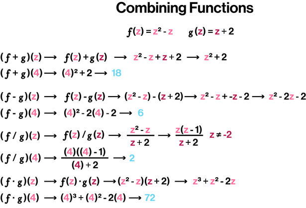
Functions can be combined by addition, subtraction, multiplication, or division.
Linear Functions


Linear Functions: Functions that produce a straight line graph.

Constant Functions: Functions of the form f(x)=b. The graph of a constant function is a horizontal line.

Vertical line graphs are not produced by functions. Vertical line graphs fail the vertical line test.

The range of a linear function is dependent on whether the equation of the function is f(x)=mx+b or f(x)=b.
Variation

Direct Variation: f(x) is proportional to x. As x increases, f(x) increases. As x decreases, f(x) decreases.
Inverse Variation: f(x) is inversely proportional to x. As x increases, f(x) decreases. As x decreases, f(x) increases.
"k" is the constant of proportionality
Systems of Equations in Two Variables
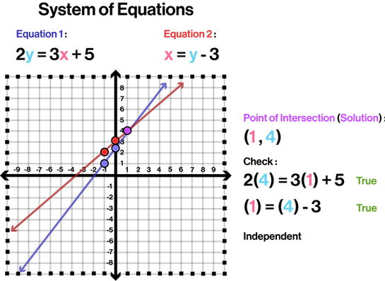


System of Equations: Two or more equations, in two or more variables, for which a common solution is sought.
Solution of a System: A solution that makes all the equations in the system true.
Graphing, substitution, and elimination are three methods used to solve systems of equations in two variables.


Consistent System of Equations: A system of equations that has at least one solution.
Inconsistent System of Equations: A system of equations that has no solution.
Dependent (Systems of Two Equations): One equation is a multiple of the other. Both equations produce the same graph.
Independent (Systems of Two Equations): Neither equation is a multiple of the other. The equations produce different graphs.
Systems of Equations in Three Variables

Systems of equations in three variables can be solved using the elimination method.

Dependent (Systems of Three Equations): A set of equations is dependent if at least one equation can be expressed as a sum of multiples of other equations in the set.
Matrices

Matrix: A rectangular array of numbers. Matrices are composed of horizontal rows and vertical columns. Matrices are named using a capital letter.

Elements: The individual numbers of a matrix. Elements are labeled using a lowercase letter followed by their row and column numbers.

Matrices with the same dimensions can be added or subtracted from each other.

Scalar: A real number that multiplies a matrix.
Scalar Product: The product of a matrix and a real number.
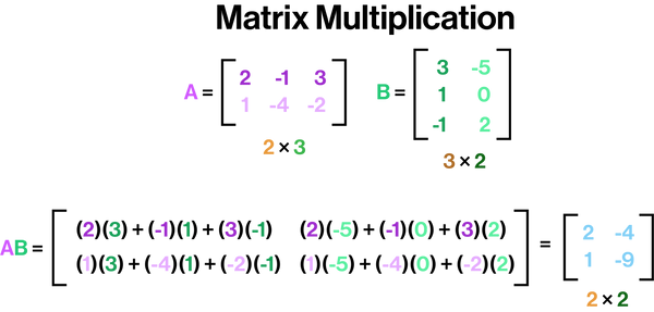
Two matrices can be multiplied when the number of columns of the first matrix is equal to the number of rows of the second matrix. Matrix multiplication is not commutative. Each element of the product matrix is the sum of several products.

A matrix can correspond to a system of equations.
Matrices can be used to solve systems of equations; however, these calculations typically require a graphing calculator.


Determinant: A descriptor of a square matrix.
Inequalities

Inequalities can contain functions.

Compound Inequalities: A mathematical sentence where two or more inequalities are joined by the word “and” or the word “or.”
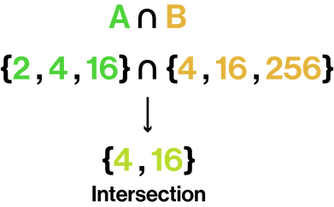
Intersection (∩) (and): The elements that are shared between two sets.

Conjunction (∩) (and): A mathematical sentence for which two or more inequalities are joined by the word “and.”

Disjoint (∅): No elements are shared between the sets.


Union (∪) (or): The elements that belong to set A and/or set B.

Disjunction (∪) (or): A mathematical sentence for which two or more inequalities are joined by the word “or.”
.png)
The domain of a function can be represented using set-builder and/or interval notation.

Only nonnegative numbers have square roots that are real numbers. Therefore, to find the domain of a radical function, an inequality must be solved.


The solution of an absolute value equation can be determined using the absolute value principle.


.png)
The solution to an absolute value inequality can be determined using the absolute value principle for inequalities.

When graphing a linear inequality on a coordinate plane, the type of line used is dependent on the inequality symbol used.


Linear Inequality: An inequality whose related equation is a linear equation.
Half-plane: A coordinate plane that is split into two regions. The shaded region of a half-plane contains all the solutions to a given linear inequality.
Boundary: The straight line that splits a coordinate plane into two half-planes.


Systems of linear inequalities can be solved by graphing the linear inequalities on a coordinate plane and determining the region of overlap.
Radicals

Square Root: “b” is a square root of “a” if “b^2” = “a”. Every positive number has two square roots, and zero has only one square root, which is itself.


Principal Square Root (√): The nonnegative square root of a number.

Square roots of the form √a^2 are equal to the absolute value of a.


Cube Root (3√): b is the cube root of a if b^3 = a. Each real number only has one real number cube root.


Rational Exponents: Fractional exponents that are equivalent to radicals.

A radical expression can be simplified by converting it into its exponential form and applying the laws of exponents.

Radicals with the same index can be combined using the product rule for radicals.

The inverse of the product rule for radicals can be used to simplify radical expressions.

The quotient rule for radicals can be applied to a fraction under a single radical symbol. When applied, both the numerator and denominator are placed under their own radical symbol.


Rationalizing: Finding an equivalent expression that either does not contain a radical in the numerator or denominator. To rationalize, the radical containing a fraction is multiplied by one either under the radical symbol or outside of it to remove the radical from either the numerator or denominator.

Radical expressions with the same radicand and index can be added or subtracted using the distributive property.

Radical expressions can be multiplied using the distributive property.

Radical Conjugate: A corresponding radical expression that contains the inverse operation.
To rationalize a numerator or denominator with two terms, a conjugate is used.

If radical terms in quotients and products have different indices, they can be simplified by converting them to exponential notation and applying the laws of exponents.

Radical Equation: An equation that contains a variable under a radical symbol.
Complex Numbers
Complex-number System: A number system that includes the real-number system and also includes negative numbers with defined square roots.

Imaginary Numbers: Expressions that contain “i.”
The imaginary number “i” can be used to define the square root of a negative number.

Complex numbers can be added and subtracted using the associative, commutative, and distributive laws.

The number “i” must be removed from each radical before applying the product rule for radicals.

The conjugate of the denominator is used when dividing complex numbers.
Quadratic Functions


Quadratic Function: A second-degree polynomial function in one variable.


The principle of square roots can be used to solve equations of the form x^2 = a.

Completing the Square: Adding a constant to an expression so that the sum is a perfect square. This method can be used to solve any quadratic equation.


Quadratic Formula: A formula used to solve quadratic equations.

The discriminant of the quadratic formula can be used to determine possible solutions.

A quadratic equation can be found by using solutions.


Some equations can be reduced to a quadratic form.

f(x) = x^2 is the most basic quadratic function. All quadratic functions produce a graph that is a parabola.

The coefficient of x^2 affects the parabola’s direction and width.
%5E2.png)
%5E2%2Bk.png)
Quadratic functions can appear in various forms.


Quadratic functions of the form ax^2 + bx + c can be converted to the form a(x - h)^2 + k by using a method similar to completing the square.


Vertex: The turning point of a parabola.
Minimum: The lowest point on a parabola.
Maximum: The highest point on a parabola.
Line of Symmetry: A line that goes vertically through the vertex. The line of symmetry reflects the two halves of a parabola.
Polynomial and Rational Inequalities


Polynomial inequalities can be solved by determining the x-intercepts and graphing.

Rational inequalities can be solved by testing intervals.
Composite and Inverse Functions

Composite Function: A function within one or more functions.

Inverse Relation: A relation formed by swapping the members of the domain and the members of the range of a relation.

One-to-One Functions: Functions for which different inputs have different outputs. The inverse of a one-to-one function is also a function.

Horizontal Line Test: It is impossible for a horizontal line to intersect a one-to-one function’s graph more than once.

f^-1(x): The inverse of the function f(x).

Finding the inverse of a function requires conversions.

The graph of an inverse function is the reflection of the original function across the y=x line.

A composite function composed of a function and its inverse is equal to x.
Exponential and Logarithmic Functions


Exponential Function: A function of the form f(x)=a^x. a, the base, is a positive constant other than one, and x is any real number. The inverse of an exponential function is a logarithmic function.


Logarithmic Function: A function of the form f(x)=logax. a is a positive constant other than 1, and x is greater than zero. The inverse of a logarithmic function is an exponential function.


The special properties of logarithms are used to manipulate and solve equations.


The principles of exponential and logarithmic equality are needed to solve exponential and logarithmic equations.

Logarithmic equations are converted to their equivalent exponential form when solving.


Common Logarithm: A base 10 logarithm.
Natural Logarithm: A base e logarithm.

A conversion formula can be used to convert a logarithm to a different base.
Conic Sections

Conic Section: A curve that is the result of a plane intersecting a cone.

Parabola: The graph of a quadratic equation.

Circle: A set of points in a plane that are a fixed distance, the radius, from the center (h,k).


Ellipse: A set of points in a plane where the sum of the distances from two fixed points, foci, is constant.


Hyperbola: A set of points in a plane whose absolute value of the difference of their distances from the foci is constant.
Nonlinear Systems of Equations

Nonlinear systems of equations can be solved by graphing, substitution, or elimination.